Symmetric Network with Dual-vehicle Attributes Augmentation

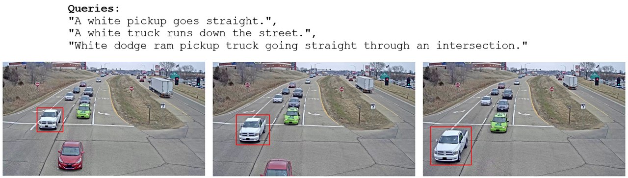
This was my first large-scale research project, and my first run at the AI City Challenge. The task, Track 2 of the 7th AI City Challenge (CVPR 2023), is retrieving the right vehicle track from a natural-language description: given a sentence like “a gray SUV turns left at a busy intersection,” find the matching video track among thousands. My solution, SNDA (Symmetric Network with Dual-vehicle Attributes Augmentation), reached 35.44% MRR, 7th place on the leaderboard.

Why the task is hard

Natural-language vehicle retrieval sits between video understanding and fine-grained re-identification, and it inherits the worst of both. Three problems make it genuinely difficult:

1. Ambiguous, information-poor queries. A single sentence rarely pins down a vehicle. “A white sedan goes straight” matches hundreds of tracks.
2. Tiny inter-class variation. Vehicles with different identities routinely share appearance and motion attributes, so the visual signal that separates them is thin.
3. Data scarcity. There simply isn’t much annotated track/vehicle data to train a robust cross-modal model, and image-query re-identification pipelines don’t transfer cleanly to text queries.

Architecture

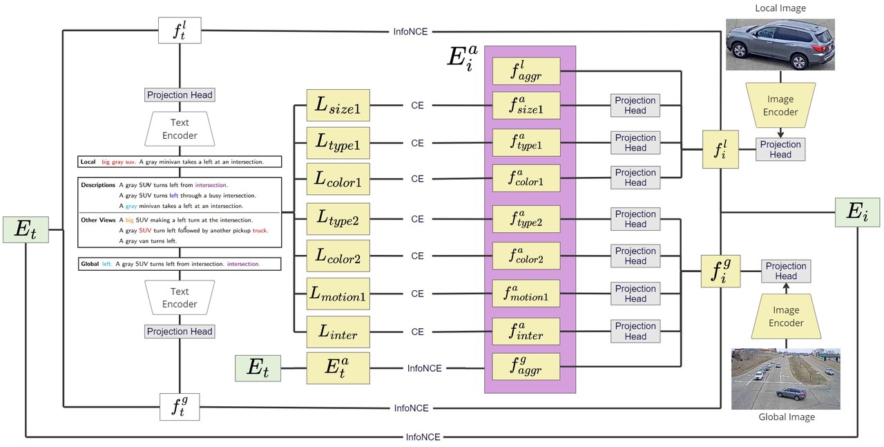
SNDA adapts the symmetric SSM design and uses four branches to capture local and global representations of each modality. Text features come from a frozen RoBERTa; visual features from an EfficientNet-B2 backbone. The idea is that local features carry instance detail (the cropped vehicle, the augmented subject phrase) while global features carry context (the whole motion image, the full sentence with location cues), and aligning both gives the model two complementary views of the same track.

Cross-modal representation learning

Each backbone embedding passes through a small projection head before alignment. The two text heads share a layer-normalized form, and the two visual heads a batch-normalized one:

$$ f_t = g_t(h_t) = W_2\,\sigma\!\big(\mathrm{LN}(W_1 h_t)\big), \qquad f_i = g_i(h_i) = W_2\,\sigma\!\big(\mathrm{BN}(W_1 h_i)\big) $$

where $h$ is a backbone embedding and $\sigma$ is ReLU. The local and global text features are concatenated into the language representation $E_t = [\,f_t^l \,\|\, f_t^g\,]$, and likewise the visual features into $E_i = [\,f_i^l \,\|\, f_i^g\,]$. Alignment then happens at four levels: the two local/global pairs, the fused pair $\langle E_i, E_t\rangle$, and an augmented pair introduced below.

Modeling motion without a video model

Every camera in the dataset is static and its background is stable, which I turned into a shortcut. Instead of a video transformer, I collapse each track into a single motion map. First average all frames into a clean background,

$$ B = \frac{1}{N}\sum_{i=1}^{N} F_i, $$

then paste the cropped vehicle from each frame’s bounding box back on top. Because boxes from consecutive frames overlap and clutter the image, I skip any box whose IoU with the previous one exceeds a threshold $T = 0.05$. The result is one motion-bearing image the visual branch can consume cheaply, capturing the vehicle’s trajectory without ever running a temporal model.

The dual-vehicle attribute system

The core idea: many queries describe two nearby vehicles, and that second vehicle is free supervision. I extract attributes by frequency-analyzing the dataset vocabulary and grouping the most common words into categories: vehicle type (suv, sedan, truck, van), color (red, blue, black, white, and a merged gray/grey/silver), size (small, mid-sized, large), motion (left, right, stop, else go straight), and an intersection flag for long-distance scene context.

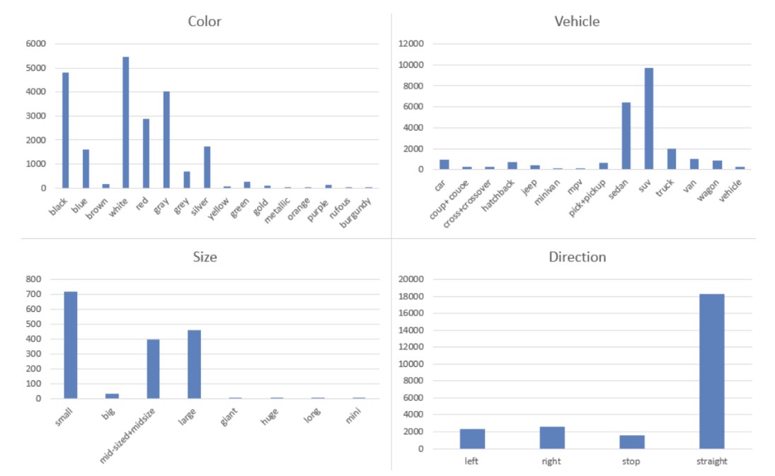
Critically, type and color come in pairs. Many sentences name the target and a nearby vehicle, so I prioritize finding two same-category words that co-occur in one query, yielding type1/type2 and color1/color2 (with color2 discarded if no type2 is found). Motion and size are extracted once as motion1 and size1. Because each attribute is mined across a shuffled, merged set of every description of a scene, the value pulled in can differ from the words in any single query, which adds detail rather than echoing it.

	Example
Primary descriptions	A gray SUV turns left from intersection.
	A gray SUV turns left through a busy intersection.
	A gray minivan takes a left at an intersection.
Other camera views	A big SUV making a left turn at the intersection.
	A gray SUV turn left followed by another pickup truck.
	A gray van turns left.

Attributes are mined across the primary descriptions and the descriptions of the same scene from other cameras. Here size (big), a second type (truck), and the intersection flag all surface from views beyond the primary sentence.

These attributes drive three mechanisms.

Text augmentation. Extracted attributes are prepended (and, for location, appended) to two sampled queries to enrich sparse descriptions, separately for the local and global text inputs.

Input	Augmented query
Local	big gray suv. A gray minivan takes a left at an intersection.
Global	left. A gray SUV turns left from intersection. intersection.

Subject augmentation (size + color + type) on the local input; motion and location augmentation on the global input.

Visual attribute heads. Seven projection heads predict the attributes directly from the visual features. For an attribute with $n_{attr}$ categories I build a one-hot label of length $n_{attr}+1$, reserving the extra slot for missing or out-of-vocabulary values so “unknown” is a first-class class rather than noise. The heads are trained with cross-entropy, forcing the visual side to learn explicit attribute signals it can match against the text.

Augmented representation pair. The visual attribute predictions are fused with the visual features into an augmented vector $E_i^a$, paired with a projected language vector $E_t^a$, giving the fourth and most attribute-aware alignment pair.

Loss functions

Every visual-language pair is aligned with a symmetric InfoNCE loss. For a batch of $N$ pairs, the two directions are

$$ \mathcal{L}_{t2i}^{z} = -\frac{1}{N}\sum_{i=1}^{N}\log \frac{\exp\!\big(\cos(z_{\text{text}}^i, z_{\text{img}}^i)/\tau\big)} {\sum_{j=1}^{N}\exp\!\big(\cos(z_{\text{text}}^i, z_{\text{img}}^j)/\tau\big)}, \qquad \mathcal{L}_{\text{SNCE}}^{z} = \tfrac{1}{2}\big(\mathcal{L}_{t2i}^{z} + \mathcal{L}_{i2t}^{z}\big), $$

with $\mathcal{L}_{i2t}^{z}$ defined symmetrically and $\tau$ a learned temperature. The representation loss sums this over all four pairs,

$$ \mathcal{L}_{\text{rep}} = \sum_{z\in\mathcal{Z}} \mathcal{L}_{\text{SNCE}}^{z}, \qquad \mathcal{Z} = \big\{\langle f_i^l, f_t^l\rangle,\ \langle f_i^g, f_t^g\rangle,\ \langle E_i, E_t\rangle,\ \langle E_i^a, E_t^a\rangle\big\}, $$

and the seven attribute heads contribute an averaged cross-entropy term, giving the total objective:

$$ \mathcal{L}_{\text{aug}} = \frac{1}{7}\sum_{attr}\mathcal{L}_{attr}^{a}, \qquad \mathcal{L} = \mathcal{L}_{\text{rep}} + \mathcal{L}_{\text{aug}}. $$

Post-processing

At inference, two relationship terms refine the similarity matrix. Long-distance modeling detects intersections (in text via the intersection flag; in video by checking whether a vehicle stays roughly still across $n$ frames) and scores their agreement as $S_l$. Short-distance modeling scores vehicle-to-vehicle relationships by matching the local features of every vehicle in a track against the query, giving $S_r$. The final matrix combines the four learned similarities with both terms:

$$ S = \sum_{z\in\mathcal{Z}} S_z + \alpha S_r + \beta S_l, \qquad \alpha = 1,\ \beta = 0.2. $$

Dataset and metrics

The track uses a variation of CityFlow-NL: 666 target vehicles across 3,598 single-view tracks from 46 calibrated cameras, each annotated with three distinct natural-language descriptions, for 2,155 training tracks plus a held-out 184 query/track test split. Descriptions cover color, maneuver, traffic scene, and relations to other vehicles.

Performance is the official Mean Reciprocal Rank, with Recall@5 and Recall@10 as secondary metrics:

$$ \mathrm{MRR} = \frac{1}{|Q|}\sum_{i=1}^{|Q|}\frac{1}{\mathrm{rank}_i}, \qquad \mathrm{Recall}@k = \frac{|R \cap D(k)|}{|R|}, $$

where $\mathrm{rank}_i$ is the position of the correct track for query $i$, and $D(k)$ the top-$k$ retrieved set.

Implementation. Frozen RoBERTa text encoder, EfficientNet-B2 visual backbone (ImageNet-pretrained), images resized to $228\times228$, batch size 64, 400 epochs of AdamW (weight decay $10^{-2}$, initial LR $0.01$) with a 40-epoch warm-up and a step decay every 80 epochs, all on a single NVIDIA A100-80G.

Results, and the lesson that stuck

The ablations told a two-sided story. On the validation set, every technique helped, and the final model reached 0.58 MRR / 0.87 R@5 / 0.94 R@10.

Method	MRR ↑	Recall@5 ↑	Recall@10 ↑
Baseline (symmetric net, no attributes)	0.47	0.32	0.69
+ all second-vehicle attributes	0.44	0.25	0.68
+ selected attributes (type2, color2 only)	0.45	0.60	0.87
+ NL augmentation	0.58	0.78	0.93
+ feature engineering (final)	0.58	0.87	0.94

Ablation on the validation set. Using *all* of the second vehicle's attributes hurts (size2 and motion2 are too sparse); keeping only type2 and color2 recovers it, and text augmentation drives the biggest jump.

But on the test set, the same natural-language augmentation that helped validation actually hurt: the model had learned validation-specific quirks and failed to cross the domain gap. Only feature engineering, ensembling, and post-processing recovered the score, to the 0.35 MRR that placed 7th.

Method	MRR ↑	Recall@5 ↑	Recall@10 ↑
Baseline	0.23	0.33	0.50
+ selected attributes	0.25	0.44	0.57
+ NL augmentation	0.23	0.36	0.51
+ feature engineering	0.24	0.39	0.58
Ensemble + post-processing (final)	0.35	0.53	0.64

Ablation on the test set. NL augmentation *regresses* the score here, the mirror image of the validation table, and only ensembling plus the post-processing terms close the gap.

The future direction I’d take from here is squarely domain adaptation, plus a better fusion mechanism for the augmentation signals. The full method is in the report and the code is on GitHub. This project also set the stage for TrafficVLM, my later AI City Challenge work that placed 3rd.